How To Process Over Size Data In Spark

3 Key techniques, to optimize your Apache Spark code

Jun 19, 2020 · 18 min read

Intro

A lot of tutorials evidence how to write spark lawmaking with just the API and code samples, simply they do non explain how to write "efficient Apache Spark" code. Some comments from users of Apache Spark

"The biggest challenge with spark is non in writing the transformations simply making sure they tin execute with large plenty data sets"

"The consequence isn't the syntax or the methods, it's figuring out why, when I exercise information technology this time does the execution have an 60 minutes when last time it was 2 minutes"

"big data and distributed systems tin be difficult"

In this tutorial you will learn 3 powerful techniques used to optimize Apache Spark code. At that place is no one size fits all solution for optimizing Spark, utilize the techniques discussed below to decide on the optimal strategy for your use case.

Distributed Systems

Earlier we look at techniques to optimize Apache Spark, we should understand what distributed systems are and how they work.

1. Distributed storage systems

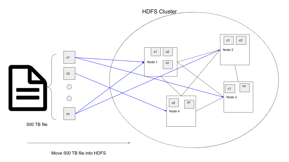
What is a distributed storage organisation? Let'due south presume we have a file which is 500 TB in size, most machines do not take the corporeality of disk space necessary to store this file. In such cases the idea is to connect a cluster of machines(aka nodes) together and split the 500 TB file into smaller (128MB by default in HDFS) chunks and spread it across the different nodes in the cluster.

For due east.k. if we desire to motility our 500 TB file into a HDFS cluster, the steps that happen internally are

1. The 500 TB file in broken downward into multiple chunks, default size of 128MB each.
2. These chunks are replicated twice, and then nosotros take 3 copies of the same data. The number of copies is called replication factor and by default is prepare to 3 to forbid data loss even if 2 nodes that contain the chunk copies neglect.
3. And so they are moved into the nodes in the cluster.
4. The HDFS system makes sure the chunks are distributed amongst the nodes in the cluster such that even if a node containing some data fails, the data can exist accessed from its replicas in other nodes.

The reason someone would desire to use distributed storage is

1. Their information is also large to exist stored in a single machine.
2. Their application are stateless and dumps all their data into a distributed storage.
3. They want to clarify large amounts of data.

2. Distributed data processing

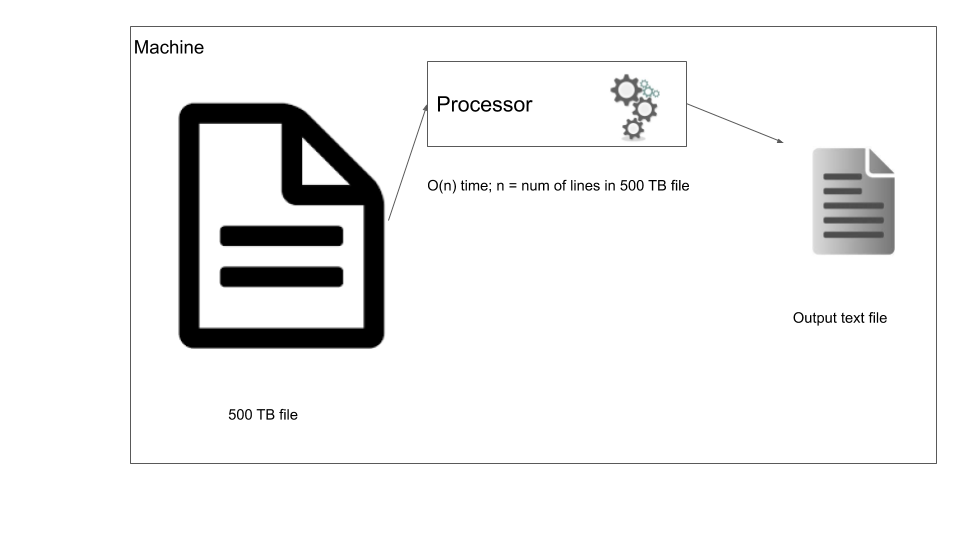
In traditional data processing you bring the data to the auto where y'all process it. In our instance, let's say nosotros want to filter out certain rows from our 500 TB file, we can run a simple script that streams through the file one line at a time and based on the filter outputs some data.

Traditional data processing

Now your script has to procedure the data file one line at a fourth dimension, but what if we tin can apply a distributed storage system and process the file in parallel? This is the foundational idea behind distributed data processing. In social club to process data that has been distributed beyond nodes nosotros use distributed data processing systems. Nearly data warehouses such every bit Redshift, Big query, Hive, use this model to process the information. Let'south consider the same instance where we have to filter our 500 TB data, but this fourth dimension the data is in a distributed storage system. In this case we employ a distributed data processing organization such as Apache Spark, the master difference here is that the data processing logic is moved to the information location where the data is processed, this way we reduce moving big information around. In the below diagram you tin run into in node 1 the processing is done inside the node and written out to disk of the same node.

Distributed information processing

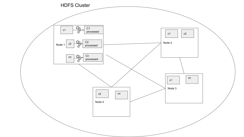
In the higher up example nosotros can see how the procedure would be much faster because the process is being run in parallel. Merely this is a very uncomplicated example where we proceed the data processing "local", that is the data is not moved over the network. This is called a local transformation.

Now that we accept a good understanding of what distributed data storage and processing is, nosotros can start to wait at some techniques to optimize Apache Spark lawmaking.

Setup

We are going to utilize AWS EMR to run a Spark, HDFS cluster.

AWS Setup

1. Create an AWS account
2. Create a pem file, follow the steps here
3. Start a EMR cluster, follow the steps here, brand sure to note downwardly y'all master's public DNS
4. Motility data into your EMR cluster using the steps shown below

SSH into your EMR primary node

            ssh -i ~/.ssh/sde.pem hadoop@<your-chief-public-dns>              # primary-public-dns sample: ec2-3-91-31-191.compute-1.amazonaws.com                      

The connection sometimes dies, so install tmux to be able to stay signed in

            sudo yum install tmux -y tmux new -south spark wget https://www.dropbox.com/s/3uo4gznau7fn6kg/Archive.zero unzip Archive.zip hdfs dfs -ls /              # listing all the HDFS folder              hdfs dfs -mkdir /input              # make a directory called input in HDFS              hdfs dfs -copyFromLocal  2015.csv /input              # copy information from local Filesystem to HDFS              hdfs dfs -copyFromLocal  2016.csv /input hdfs dfs -ls /input              # cheque to meet your copied data              wget https://www.dropbox.com/s/yuw9m5dbg03sad8/plate_type.csv hdfs dfs -mkdir /mapping hdfs dfs -copyFromLocal  plate_type.csv /mapping hdfs dfs -ls /mapping                      

Now you have moved your data into HDFS and are ready to start working with it through Spark.

Optimizing your spark lawmaking

We volition be using AWS EMR to run spark code snippets. A few things to know about spark before we start

1. Apache Spark is lazy loaded, ie it does not perform the operations until we require an output. eg: If we filter a data frame based on a sure field information technology does not get filtered immediately but only when you write the output to a file organization or the driver requires some data. The advantage here is that Spark can actually optimize the execution based on the entire execution logic before starting to process the data. So if you perform some filtering, joins, etc and then finally write the stop result to a file system, only then is the logic executed by Apache Spark.

2. Apache Spark is a distributed data processing system and open source.

In this mail service we volition be working exclusively with dataframes, although nosotros can work with RDDdue south, dataframes provide a nice tabular abstraction which makes processing information easier and is optimized automatically for us. There are cases where using RDD is beneficial, but RDD does not have the catalyst optimizer or Tungsten execution engine which are enabled by default when we utilise dataframes.

Technique 1: reduce data shuffle

The most expensive performance in a distributed arrangement such as Apache Spark is a shuffle. Information technology refers to the transfer of data between nodes, and is expensive because when dealing with large amounts of information we are looking at long wait times. Let's await at an example, start Apache spark vanquish using pyspark --num-executors=ii control

            pyspark --num-executors=              2              # num-executors to specify how many executors this spark job requires                      

            parkViolations              =              spark.read.option("header", True).csv("/input/") plateTypeCountDF              =              parkViolations.groupBy("Plate Type").count() plateTypeCountDF.explain()              # used to testify the plan before execution, in the UI we tin can just run into executed commands                      

We can use explain to view the query programme that is going to exist used to read and process the data. Here we encounter a shuffle denoted past Commutation. Nosotros aim to reduce shuffles, but there are cases where nosotros have to shuffle the data. GroupBy is i of those transformations. Since this involves a shuffle this transformation is called a wide-transformation. Permit's make Spark actually execute the operation by writing the output to a HDFS location.

            plateTypeCountDF.write.format("com.databricks.spark.csv").selection("header", True).mode("overwrite").save("/output/plate_type_count") exit()                      

Spark UI

Y'all tin view the execution of your transformation using the Spark UI. You lot can become to it as shown below. Notation: spark UI maybe slow sometimes, give it a few minutes afterwards execution to display the DAGs.

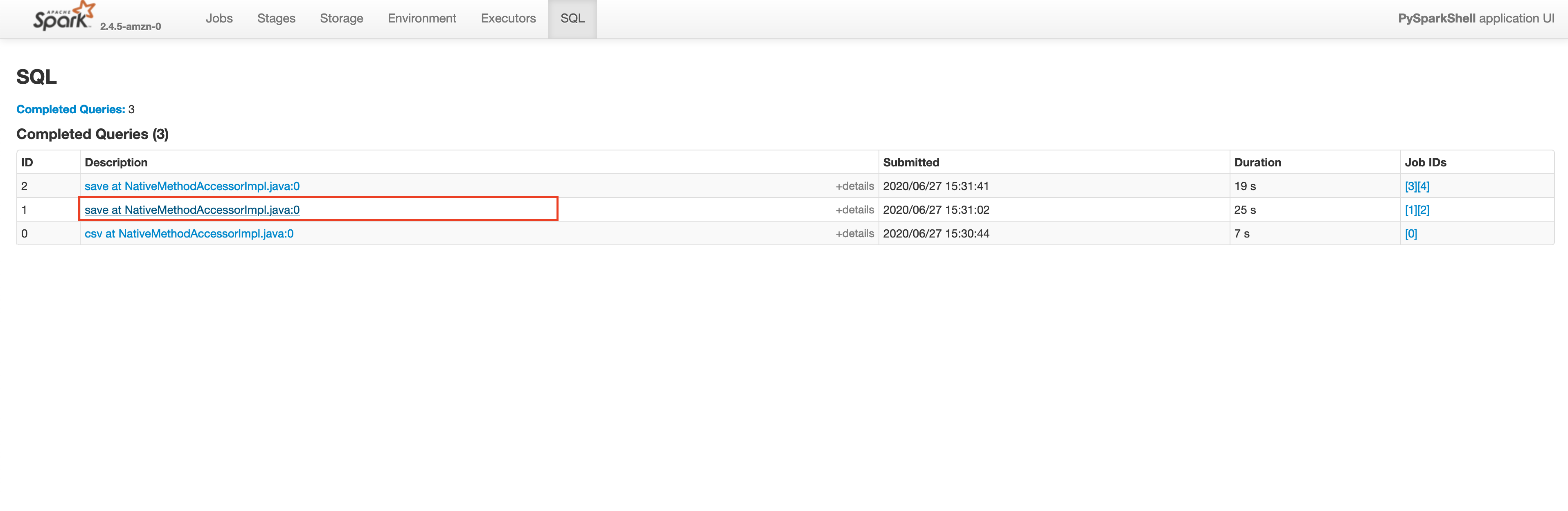
Spark History Server

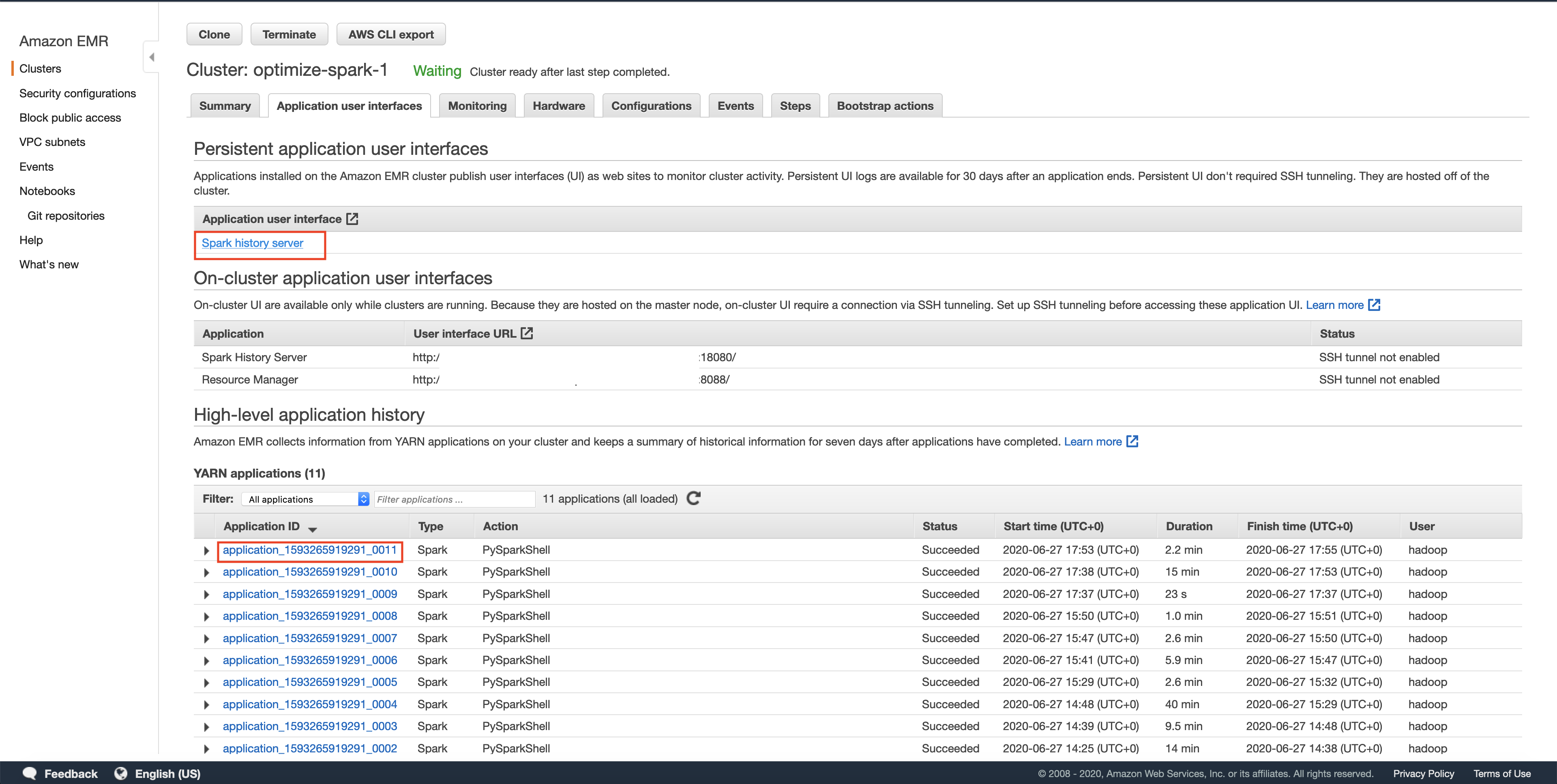
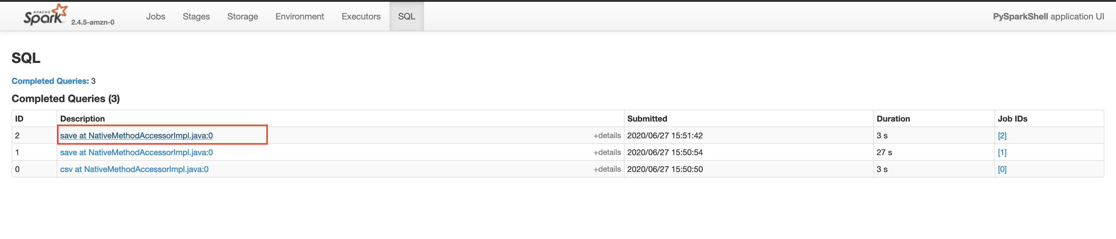
The history server will accept a listing of all the spark applications that have run. Sometimes you may have to wait for the application shown in AWS EMR UI to show upwardly on the Spark UI, we tin optimize this to be more than real time, but since this is a toy case we go out information technology every bit such. In this post we volition utilise a spark REPL(read-evaluate-impress-loop) to endeavor out the commands and exit later on competing that section. Each spark REPL session corresponds to an application. Sometimes even after quitting the spark REPL, your awarding will nonetheless be in the Incomplete applications page.

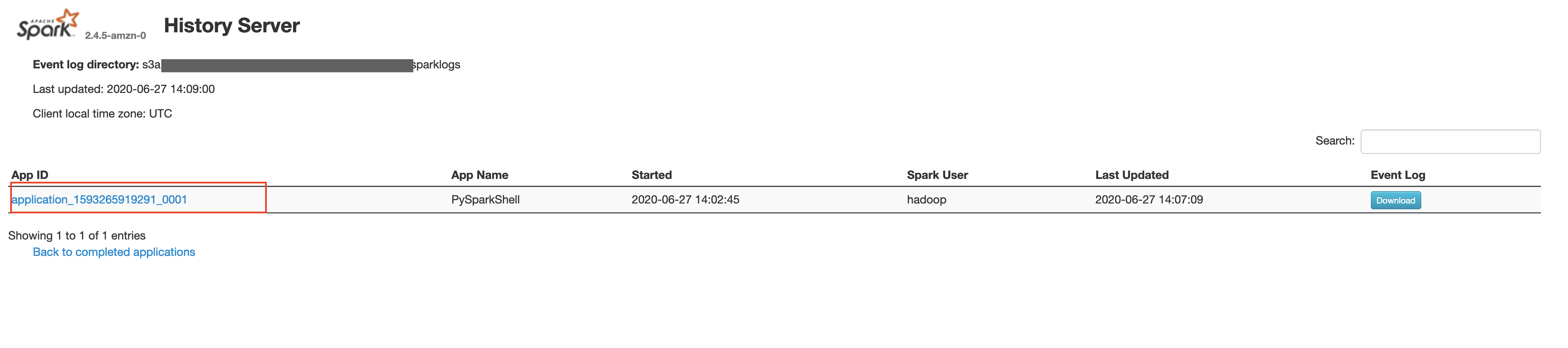
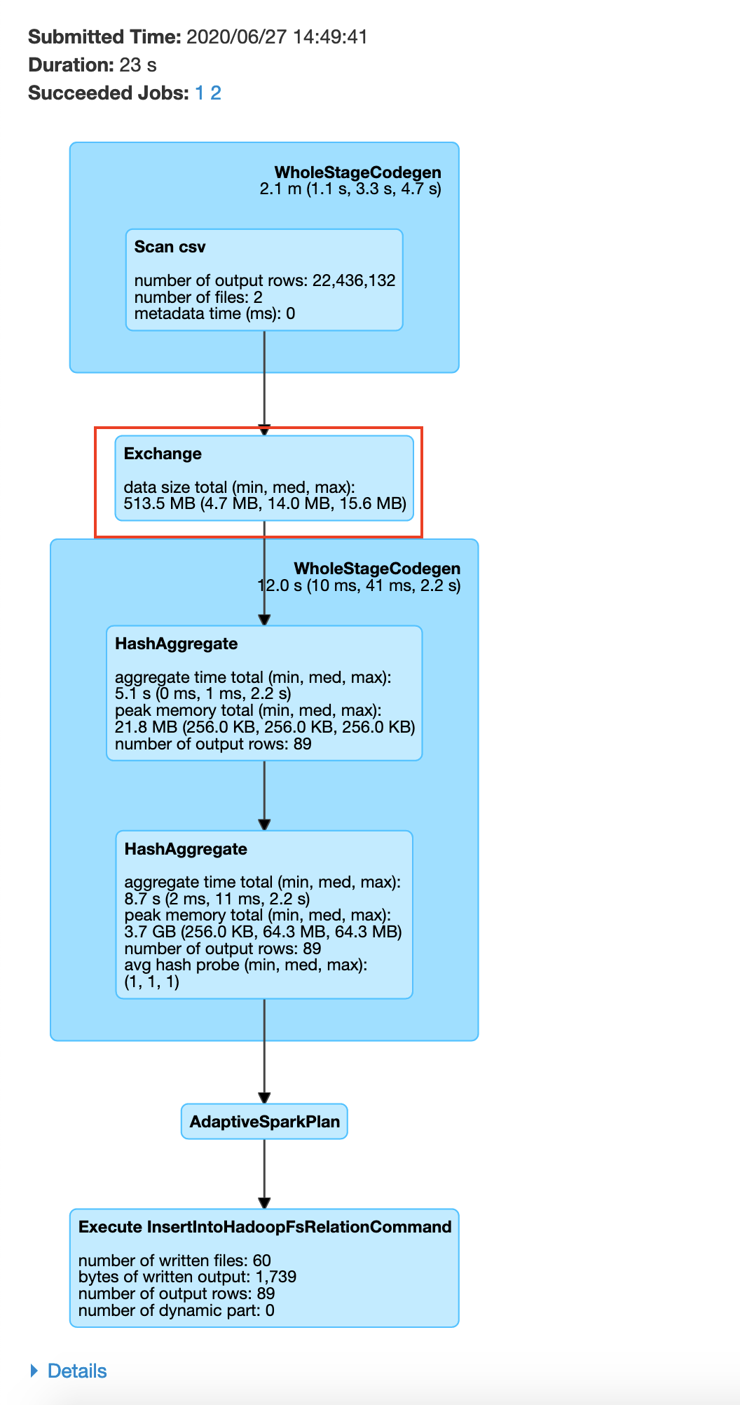
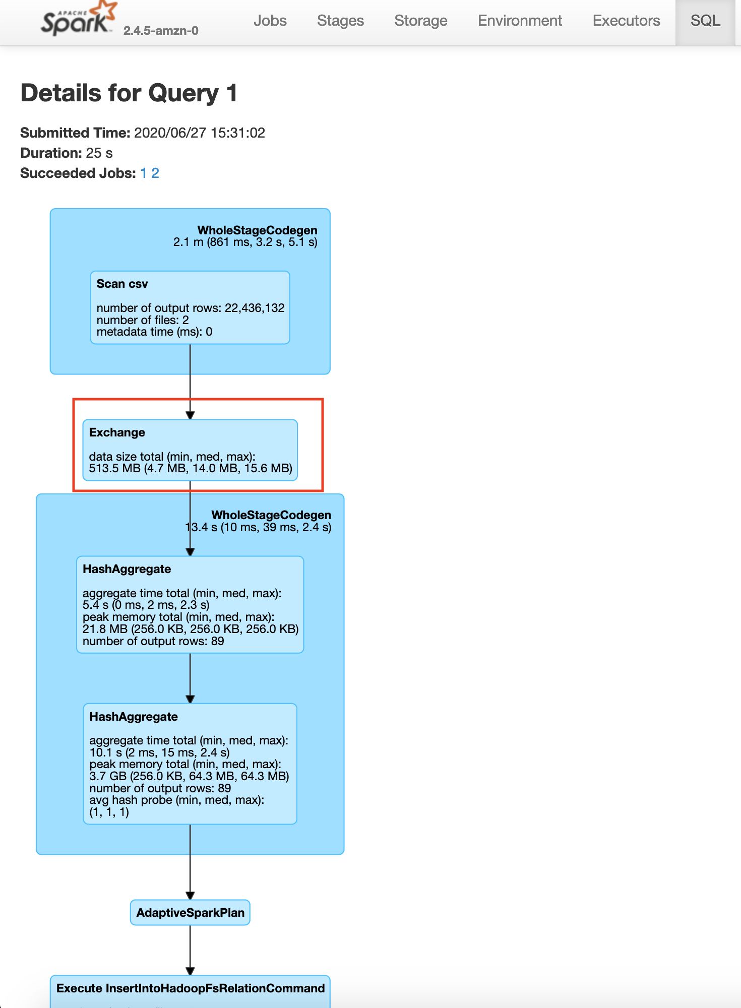
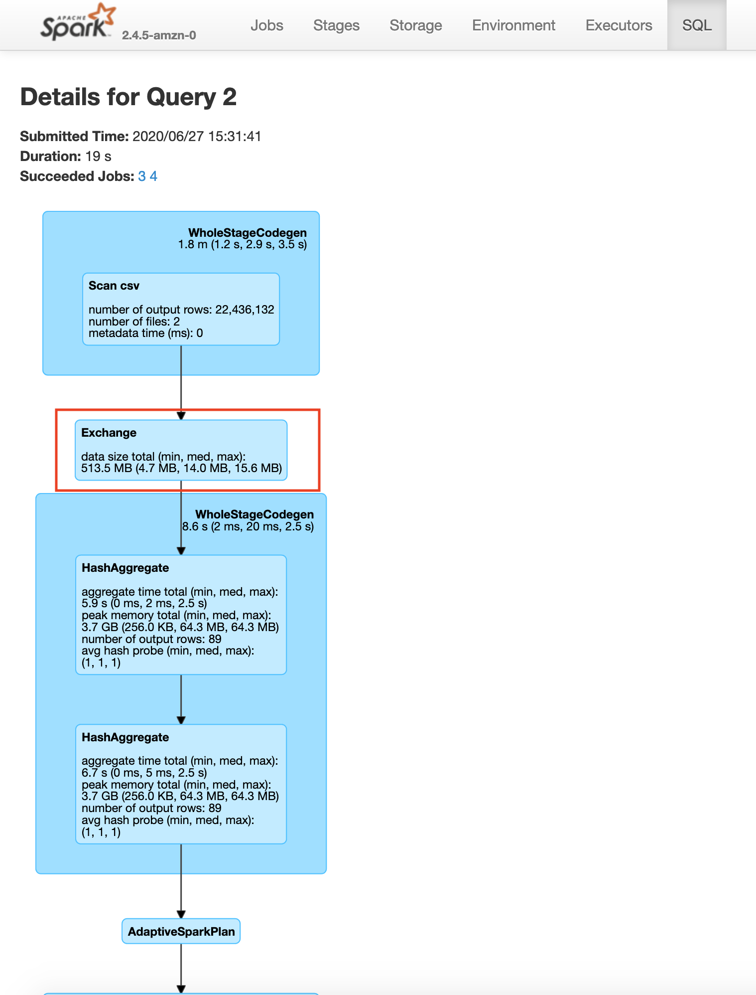
Make sure that the App ID you select in the spark history server is the latest one available in the AWS EMR's Application User Interface tab. Delight wait for a few minutes if the awarding does not testify up. This volition have y'all to the lastest Apache Spark application. In the awarding level UI, yous tin can come across the individual transformations that take been executed. Become to the SQL tab and click on the save query, every bit shown beneath.

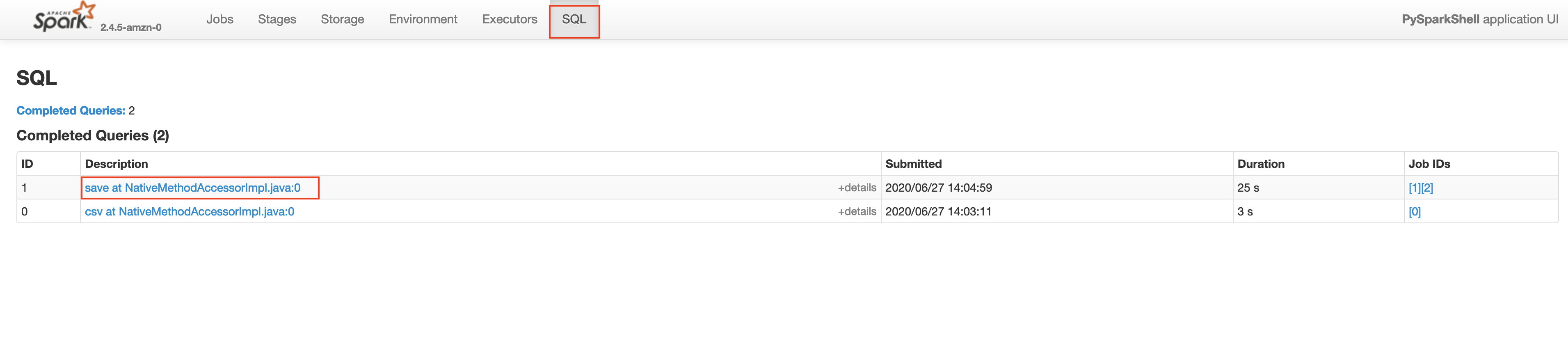
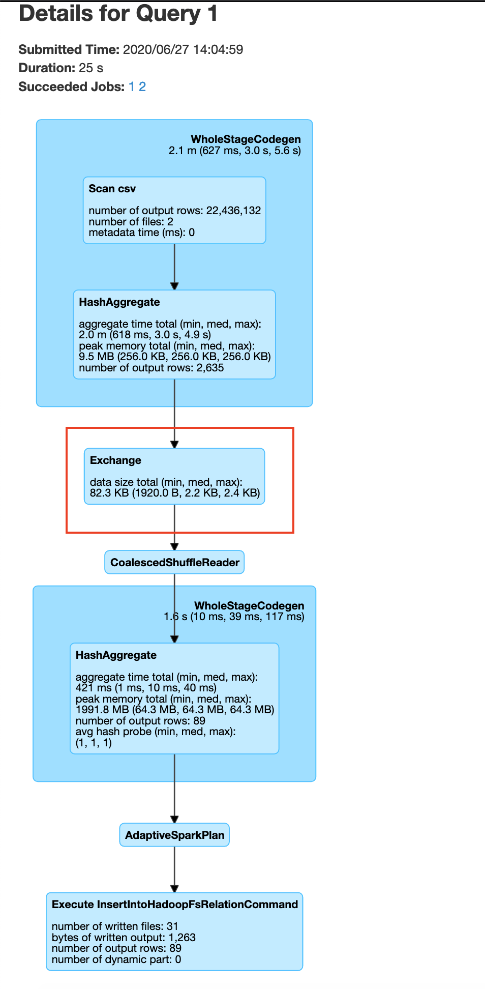
In the save query page, you will be able to run into the verbal procedure washed by the Spark execution engine. You volition observe a step in the process called exchange which is the expensive data shuffle procedure.

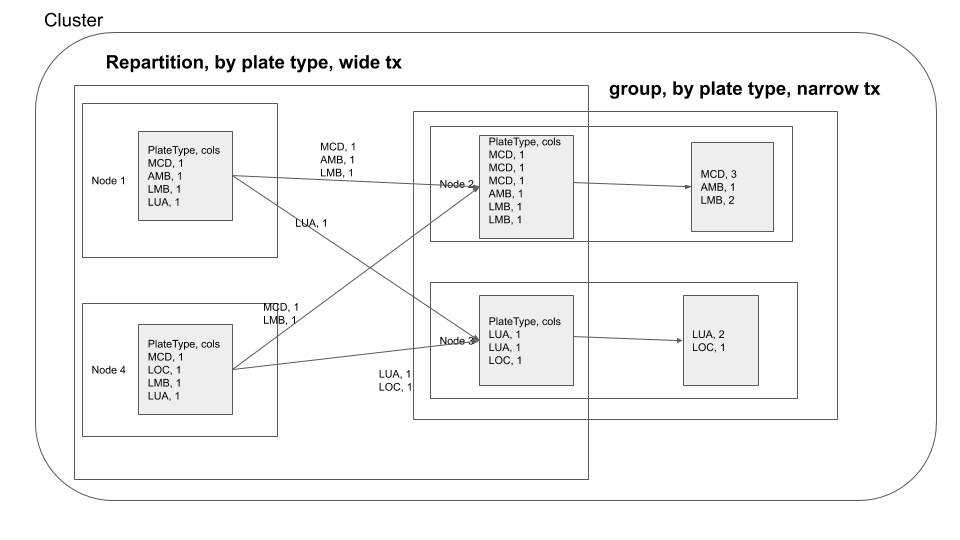
You tin can visualize the groupBy operation in a distributed cluster, as follows

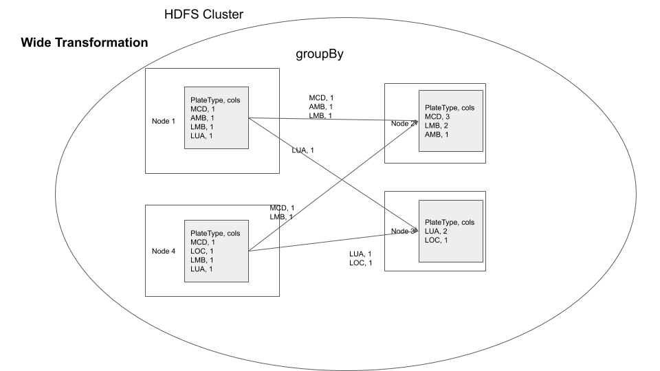
If you are performing groupBy multiple times on the same field, y'all can actually sectionalization the information by that field and have subsequent groupBy transformations use that information. So what is partitioning, partitioning is a procedure where the information is split into multiple chunks based on a particular field or we tin can only specify the number of partitions . In our instance, if nosotros partition by the field Plate Type all the rows with similar Plate Type values finish upward in the aforementioned node. This ways when we practise groupBy in that location is no demand for a data shuffle, thereby increasing the speed of the performance. This has the trade off that the data has to exist partitioned offset. Every bit mentioned earlier use this technique. If you are performing groupBy multiple times on the same field multiple times or if you demand fast query response time and are ok with preprocessing(in this case information shuffling ) the data.

            pyspark --num-executors=              two              # outset pyspark trounce                      

            parkViolations              =              spark.read.choice("header", True).csv("/input/") parkViolationsPlateTypeDF              =              parkViolations.repartition(87,              "Plate Type") parkViolationsPlateTypeDF.explicate()              # you will see a filescan to read information and exchange hashpartition to shuffle and sectionalization based on Plate Type              plateTypeCountDF              =              parkViolationsPlateTypeDF.groupBy("Plate Type").count() plateTypeCountDF.explicate()              # check the execution plan, you will come across the lesser two steps are for creating parkViolationsPlateTypeDF              plateTypeCountDF.write.format("com.databricks.spark.csv").option("header", Truthful).mode("overwrite").save("/output/plate_type_count.csv") exit()                      

You may be wondering how nosotros got the number 87, It is the number of unique plate type values in the plate type field. We got this from plate_type.csv file. If we do not specify 87, spark will by default set the number of partitions to 200(spark.sql.shuffle.partitions) which would negate the benefits of repartitioning. In your history server -> application UI -> SQL tab -> save query , you volition be able to run into the exchange happen before the groupBy as shown beneath

After the data commutation acquired by the repartition operation nosotros see that the data processing is done without moving data beyond the network, this is called a narrow transformation

Narrow Transformation

Here you repartition based on Plate Type, after which your groupby becomes a narrow transformation.

Key points

1. Data shuffle is expensive, just sometimes necessary.
2. Depending on your code logic and requirements, if you take multiple wide transformations on ane(or more) fields, y'all can repartition the information by that ane(or more than) fields to reduce expensive data shuffles in the wide transformations.
3. Check Spark execution using .explain earlier actually executing the lawmaking.
4. Check the plan that was executed through History server -> spark application UI -> SQL tab -> operation.

Technique 2. Utilise caching, when necessary

There are scenarios where it is beneficial to cache a data frame in memory and not accept to read it into memory each fourth dimension. Let's consider the previous data repartition example

            pyspark --num-executors=              ii              # start pyspark shell                      

            parkViolations              =              spark.read.choice("header", True).csv("/input/") parkViolationsPlateTypeDF              =              parkViolations.repartition(87,              "Plate Type") plateTypeCountDF              =              parkViolationsPlateTypeDF.groupBy("Plate Type").count() plateTypeCountDF.write.format("com.databricks.spark.csv").option("header", True).way("overwrite").save("/output/plate_type_count.csv")              # nosotros also practise a average assemblage              plateTypeAvgDF              =              parkViolationsPlateTypeDF.groupBy("Plate Type").avg()              # avg is not meaningful here, only used only as an aggregation example              plateTypeAvgDF.write.format("com.databricks.spark.csv").option("header", True).fashion("overwrite").save("/output/plate_type_avg.csv") exit()                      

Permit's check the Spark UI for the write functioning on plateTypeCountDF and plateTypeAvgDF dataframe.

Saving plateTypeCountDF without cache

Saving plateTypeAvgDF without cache

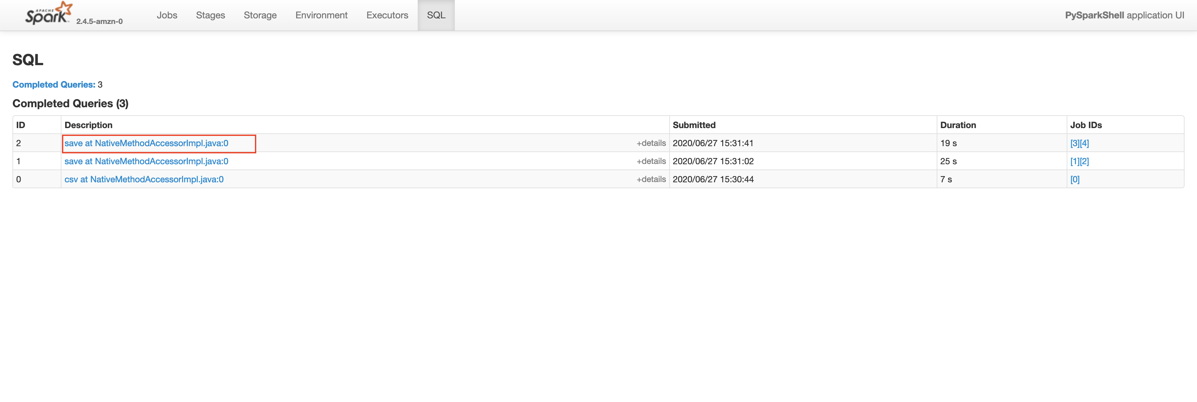
You will see that we are redoing the repartition step each time for plateTypeCountDF and plateTypeAvgDF dataframe. Nosotros can forestall the second repartition by caching the outcome of the outset repartition, as shown below

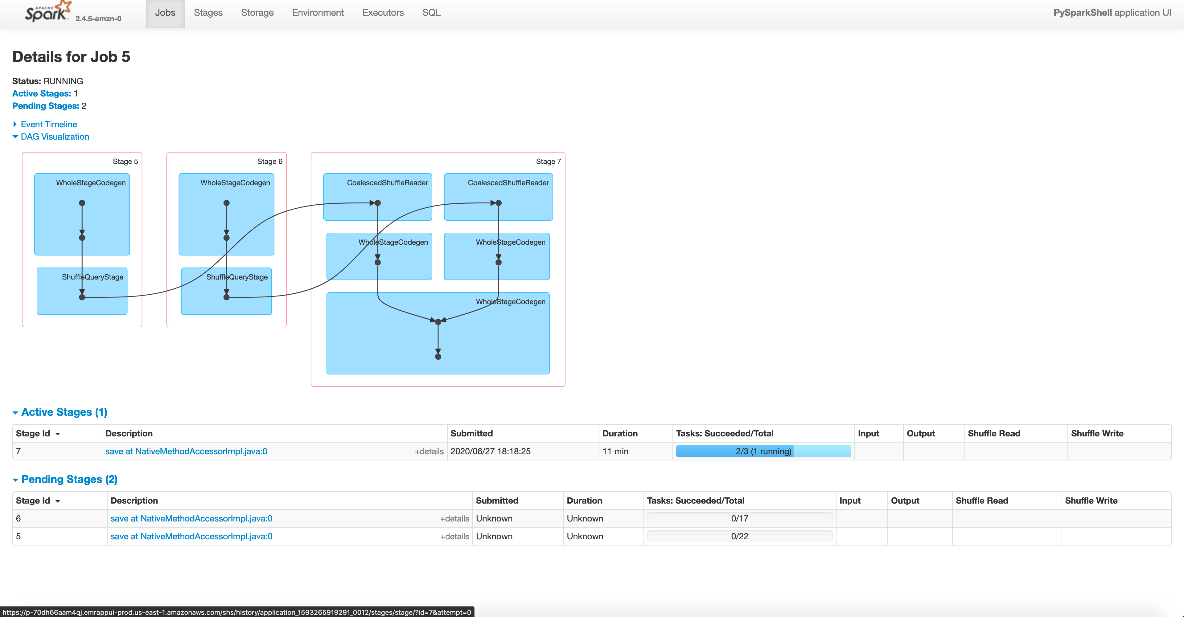
            pyspark --num-executors=              2              # start pyspark beat                      

            parkViolations              =              spark.read.option("header", True).csv("/input/") parkViolationsPlateTypeDF              =              parkViolations.repartition(87,              "Plate Type") cachedDF              =              parkViolationsPlateTypeDF.select('Plate Type').enshroud()              # nosotros are caching only the required field of the  dataframe in retentivity to keep cache size modest              plateTypeCountDF              =              cachedDF.groupBy("Plate Blazon").count() plateTypeCountDF.write.format("com.databricks.spark.csv").option("header", True).style("overwrite").salve("/output/plate_type_count.csv")              # we likewise do a average aggregation              plateTypeAvgDF              =              cachedDF.groupBy("Plate Type").avg()              # avg is not meaningful hither, merely used merely as an aggregation example              plateTypeAvgDF.write.format("com.databricks.spark.csv").option("header", True).mode("overwrite").salve("/output/plate_type_avg.csv") exit()                      

If your process involves multiple Apache Spark jobs having to read from parkViolationsPlateTypeDF y'all can besides save it to the disk in your HDFS cluster, so that in the other jobs yous can perform groupby without repartition. Allow'south check the Spark UI for the write operation on plateTypeCountDF and plateTypeAvgDF dataframe.

Saving plateTypeCountDF with cache

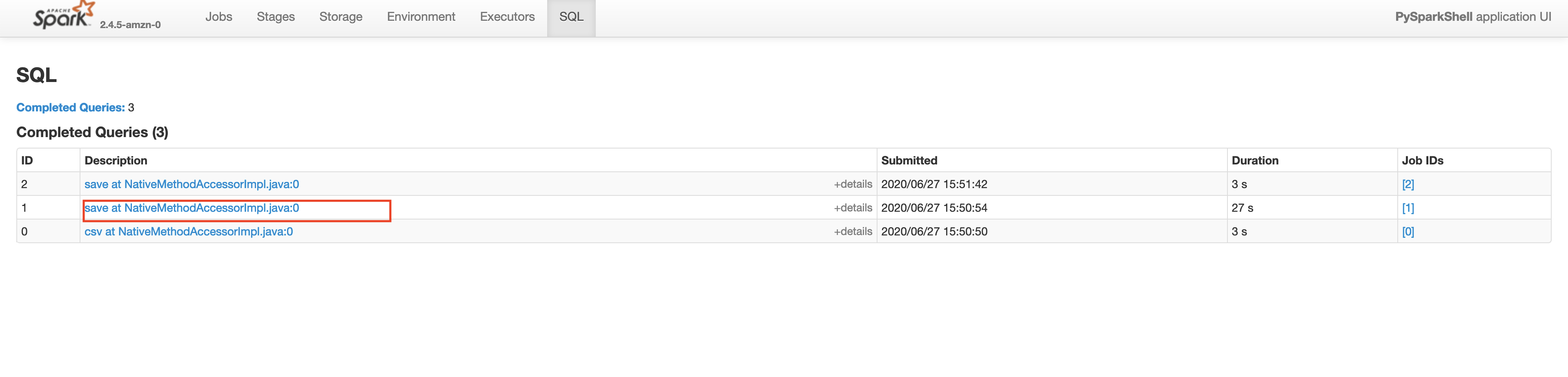
Saving plateTypeAvgDF with cache

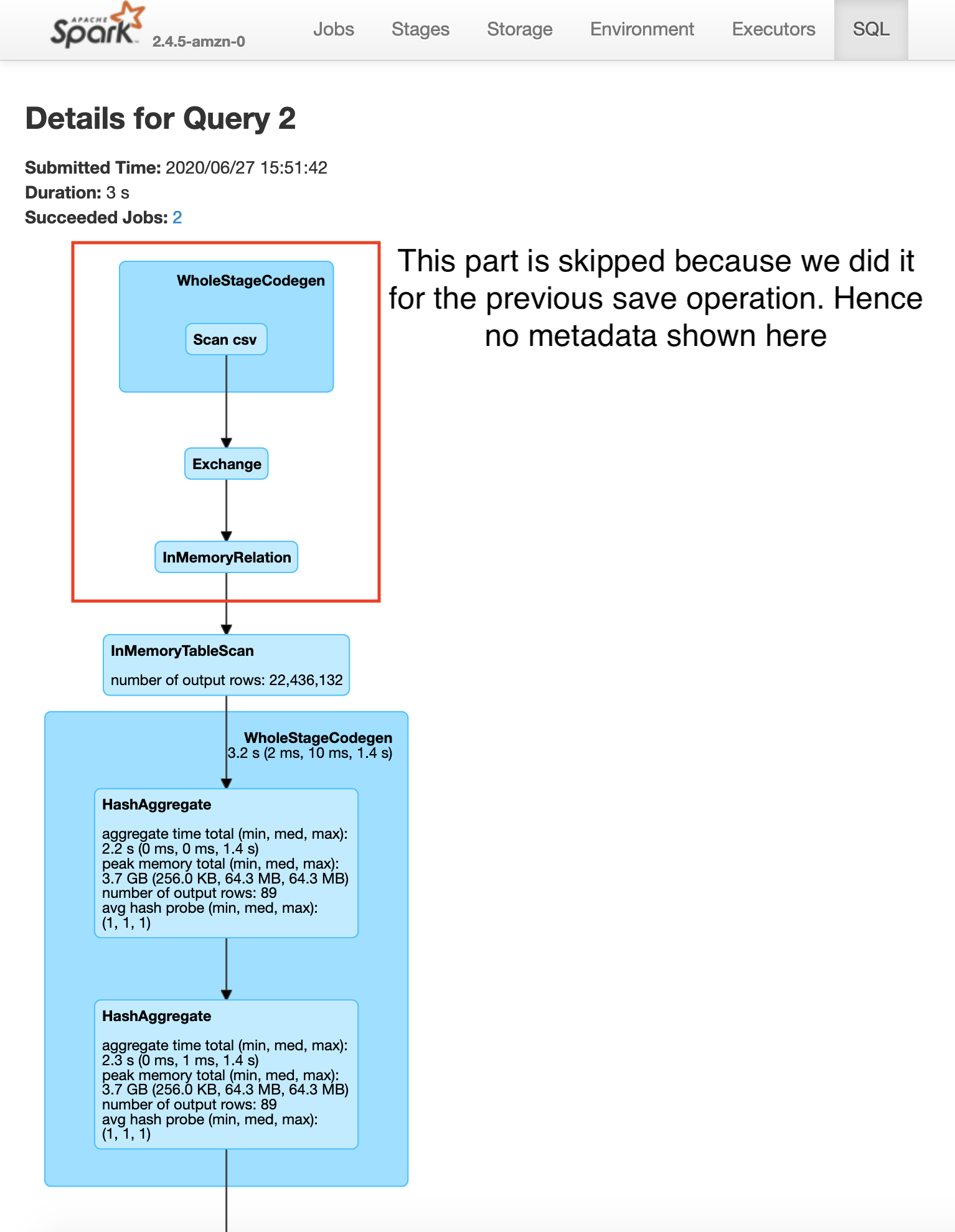
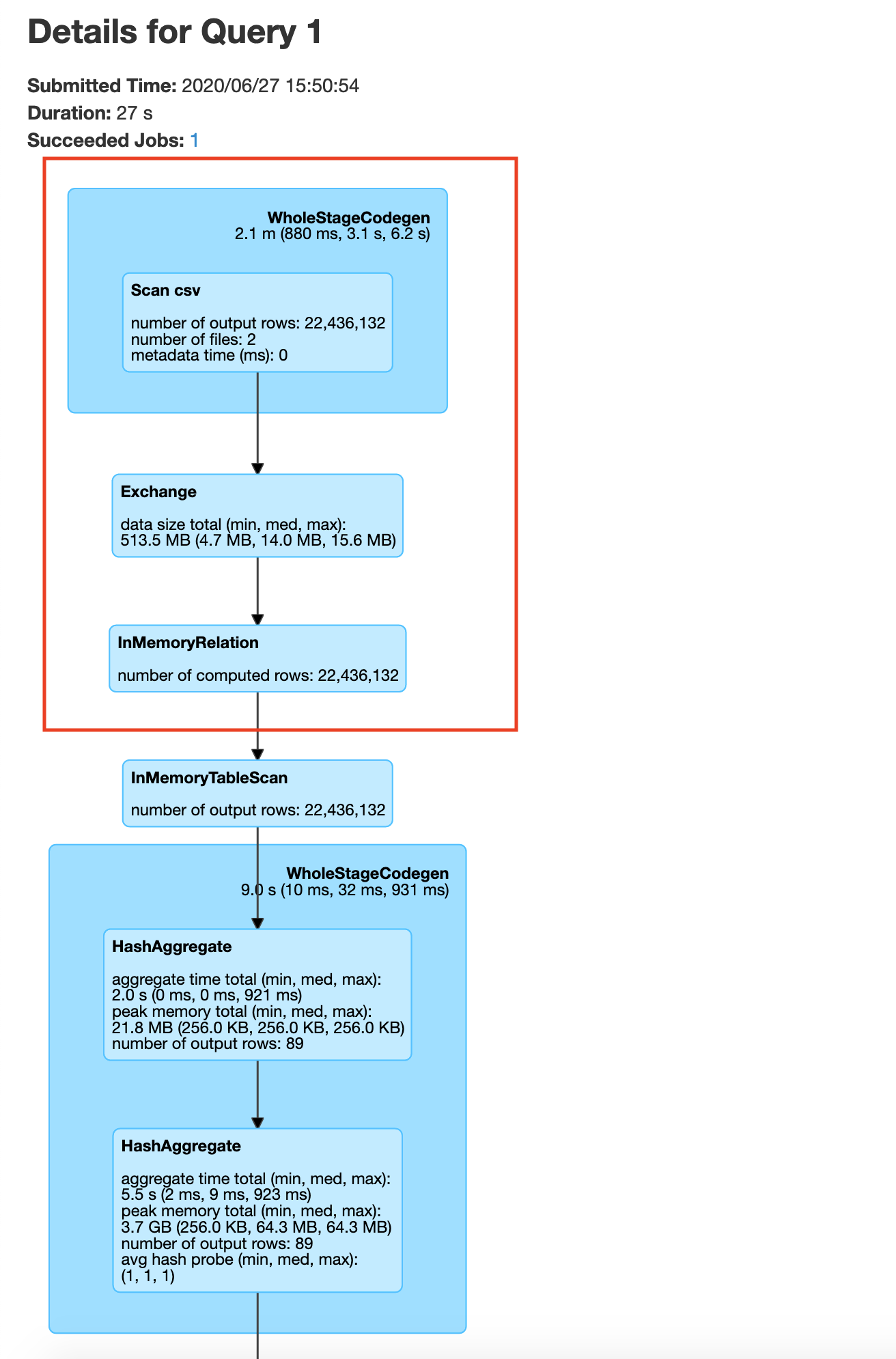
Hither you will see that the construction of plateTypeAvgDF dataframe does not involve the file scan and repartition, because that dataframe parkViolationsPlateTypeDF is already in the cluster retention. Annotation that here we are using the clusters cache memory. For very large dataframes nosotros tin utilize persist method to save the dataframe using a combination of cache and deejay if necessary. Caching a dataframe avoids having to re-read the dataframe into memory for processing, but the tradeoff is the fact that the Apache Spark cluster now holds an entire dataframe in retention.

You will likewise encounter a meaning increase in speed betwixt the 2nd salve operations in the example without caching 19s vs with caching 3s .

Y'all can visualize caching as shown below, for one node in the cluster

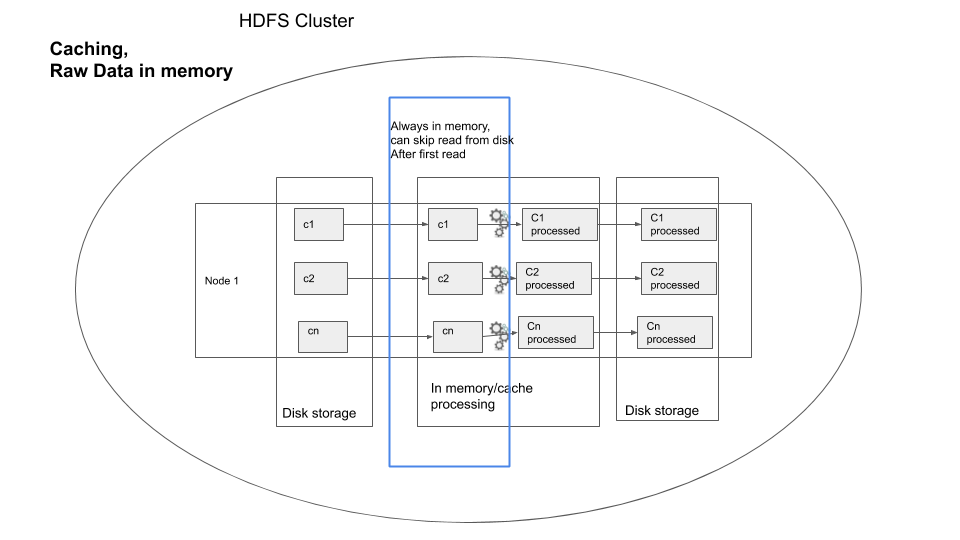
user do

Consider that you accept to save the parkViolations into parkViolationsNY, parkViolationsNJ, parkViolationsCT, parkViolationsAZ depending on the Registration State field. Volition caching assist hither, if and so how?

Key points

1. If you are using a particular data frame multiple times, try caching the dataframe's necessary columns to prevent multiple reads from disk and reduce the size of dataframe to be cached.
2. One matter to be aware of is the enshroud size of your cluster, do not enshroud data frames if non necessary.
3. The tradeoff in terms of speed is the fourth dimension taken to cache your dataframe in retentivity.
4. If you need a fashion to enshroud a data frame part in memory and part in disk or other such variations refer to persist

Technique 3. Join strategies - broadcast join and bucketed joins

1 of the most mutual operations in data processing is a join. When you are joining multiple datasets you end upwards with data shuffling because a chunk of data from the first dataset in ane node may have to be joined against some other data chunk from the 2nd dataset in another node. There are ii central techniques you can do to reduce(or fifty-fifty eliminate) data shuffle during joins.

iii.1. Circulate Bring together

Most big data joins involves joining a large fact tabular array against a small mapping or dimension table to map ids to descriptions, etc. If the mapping table is modest enough we can use broadcast bring together to motion the mapping tabular array to each of the node that has the fact tables data in information technology and preventing the data shuffle of the large dataset. This is chosen a circulate bring together due to the fact that we are broadcasting the dimension table. By default the maximum size for a tabular array to be considered for dissemination is 10MB.This is gear up using the spark.sql.autoBroadcastJoinThreshold variable. First lets consider a join without broadcast.

            hdfs dfs -rm -r /output              # costless up some space in HDFS              pyspark --num-executors=              2              # starting time pyspark shell                      

            parkViolations_2015              =              spark.read.selection("header", True).csv("/input/2015.csv") parkViolations_2016              =              spark.read.choice("header", True).csv("/input/2016.csv")  parkViolations_2015              =              parkViolations_2015.withColumnRenamed("Plate Type",              "plateType")              # elementary column rename for easier joins              parkViolations_2016              =              parkViolations_2016.withColumnRenamed("Plate Blazon",              "plateType")  parkViolations_2016_COM              =              parkViolations_2016.filter(parkViolations_2016.plateType              ==              "COM") parkViolations_2015_COM              =              parkViolations_2015.filter(parkViolations_2015.plateType              ==              "COM")  joinDF              =              parkViolations_2015_COM.join(parkViolations_2016_COM, parkViolations_2015_COM.plateType              ==              parkViolations_2016_COM.plateType,              "inner").select(parkViolations_2015_COM["Summons Number"], parkViolations_2016_COM["Issue Date"]) joinDF.explicate()              # you will see SortMergeJoin, with exchange for both dataframes, which means involves data shuffle of both dataframe              # The below join will take a very long time with the given infrastructure, exercise not run, unless needed              # joinDF.write.format("com.databricks.spark.csv").option("header", Truthful).style("overwrite").save("/output/joined_df")              exit()                      

The above process will be very tiresome, since it involves distributing ii large datasets and so joining

In order to preclude the data shuffle of two large datasets, you tin can optimize your code to enable broadcast bring together, as shown below

            hdfs dfs -rm -r /output              # free upwardly some infinite in HDFS              pyspark --num-executors=              2              # start pyspark shell                      

            parkViolations_2015              =              spark.read.pick("header", True).csv("/input/2015.csv") parkViolations_2016              =              spark.read.selection("header", True).csv("/input/2016.csv")  parkViolations_2015              =              parkViolations_2015.withColumnRenamed("Plate Type",              "plateType")              # simple column rename for easier joins              parkViolations_2016              =              parkViolations_2016.withColumnRenamed("Plate Type",              "plateType")  parkViolations_2015_COM              =              parkViolations_2015.filter(parkViolations_2015.plateType              ==              "COM").select("plateType",              "Summons Number").distinct() parkViolations_2016_COM              =              parkViolations_2016.filter(parkViolations_2016.plateType              ==              "COM").select("plateType",              "Event Date").singled-out()  parkViolations_2015_COM.cache() parkViolations_2016_COM.cache()  parkViolations_2015_COM.count()              # will cause parkViolations_2015_COM to be cached              parkViolations_2016_COM.count()              # volition cause parkViolations_2016_COM to be cached              joinDF              =              parkViolations_2015_COM.join(parkViolations_2016_COM.hint("circulate"), parkViolations_2015_COM.plateType              ==              parkViolations_2016_COM.plateType,              "inner").select(parkViolations_2015_COM["Summons Number"], parkViolations_2016_COM["Issue Date"]) joinDF.explicate()              # you will run into BroadcastHashJoin              joinDF.write.format("com.databricks.spark.csv").pick("header", True).mode("overwrite").save("/output/joined_df") exit()                      

In the Spark SQL UI you will see the execution to follow a broadcast join.

In some cases if 1 of the dataframe is modest Spark automatically switches to use broadcast join equally shown below.

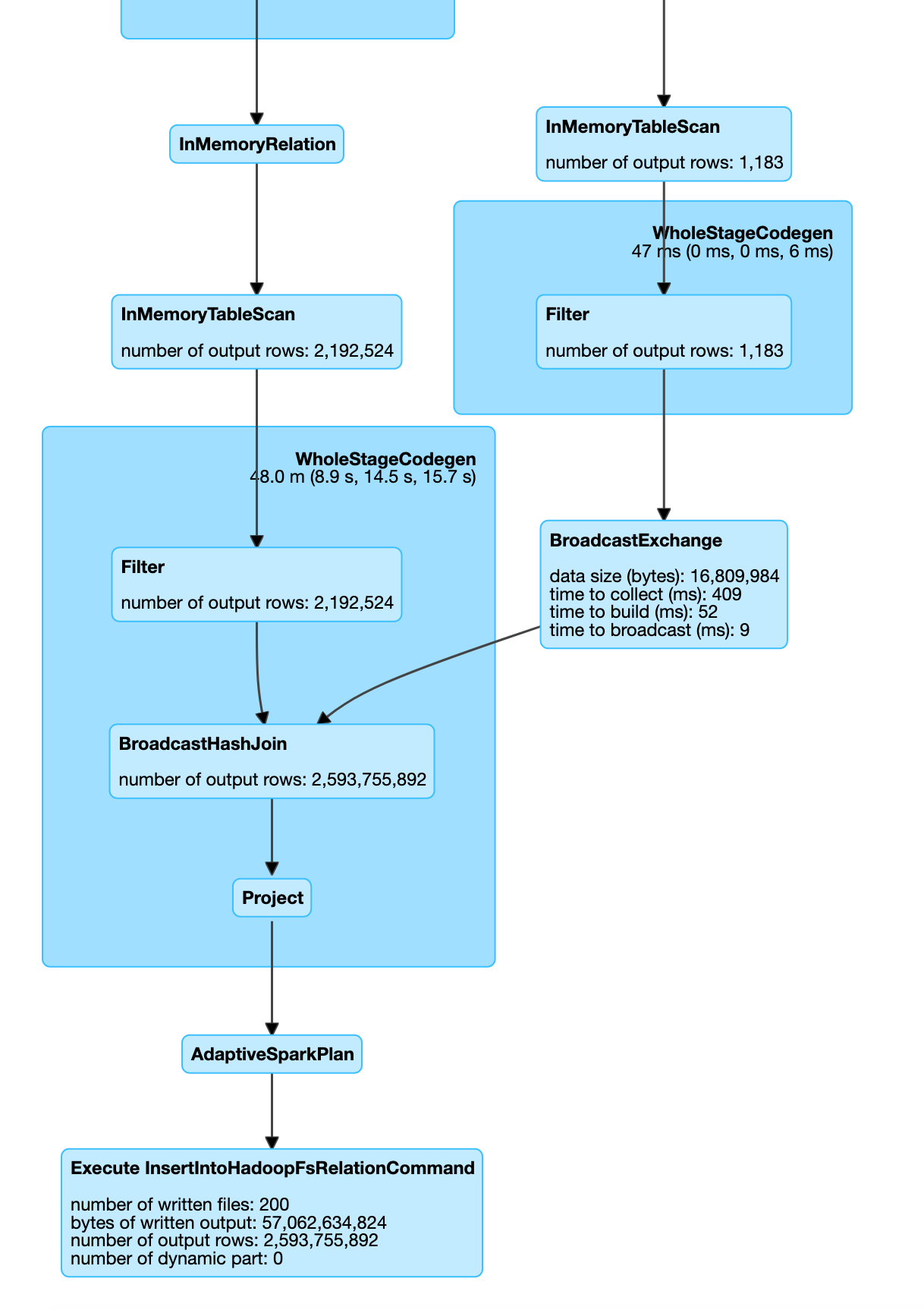
            parkViolations              =              spark.read.option("header", True).csv("/input/") plateType              =              spark.read.schema("plate_type_id Cord, plate_type String").csv("/mapping/plate_type.csv") parkViolations              =              parkViolations.withColumnRenamed("Plate Type",              "plateType")              # simple column rename for easier joins              joinDF              =              parkViolations.join(plateType, parkViolations.plateType              ==              plateType.plate_type_id,              "inner") joinDF.write.format("com.databricks.spark.csv").selection("header", True).manner("overwrite").save("/output/joined_df.csv") go out()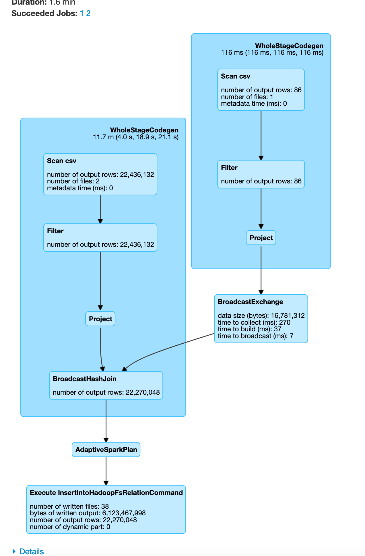                      

You can visualize this as

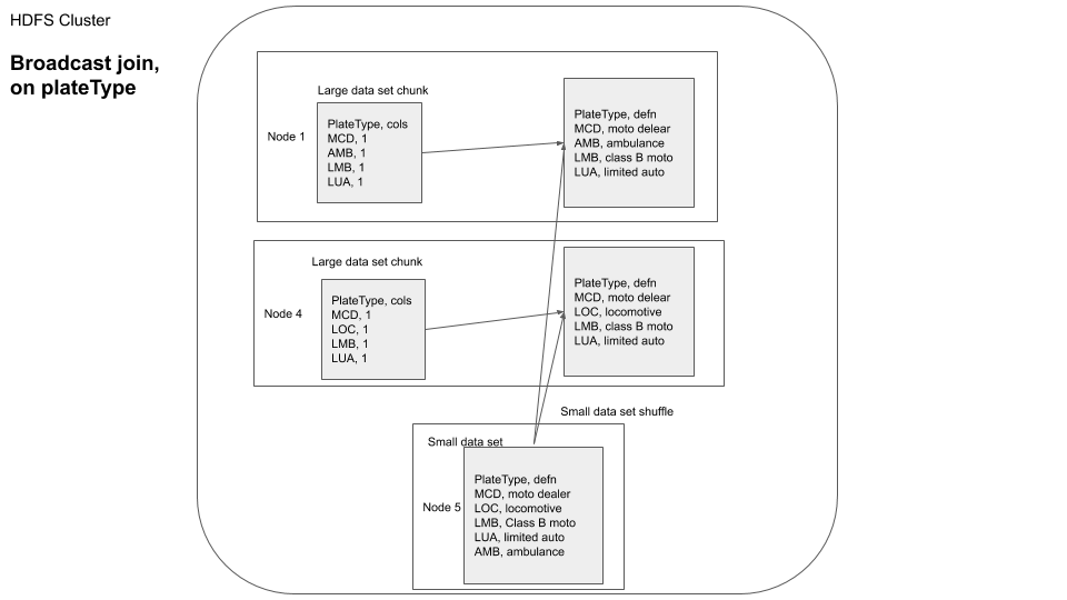
In this example since our plateType dataframe is already small, Apache Spark machine optimizes and chooses to use a circulate join. From the higher up you can see how we tin can do a broadcast join to reduce the data moved over the network.

3.2. Bucketed Bring together

In an example above nosotros joined parkViolations_2015 and parkViolations_2016, simply only kept certain columns and only after removing duplicates. What if we need to do joins in the future based on the plateType field but we might need virtually (if not all) of the columns, as required by our plan logic.

You can visualize it as shown below

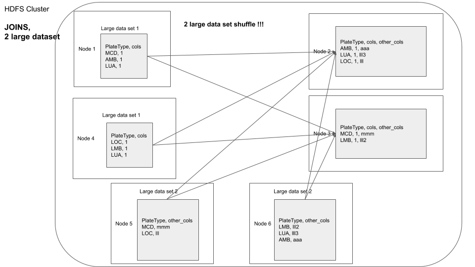
A basic approach would be to repartition ane dataframe by the field on which the join is to exist performed and so join with the second dataframe, this would involve data shuffle for the second dataframe at transformation time.

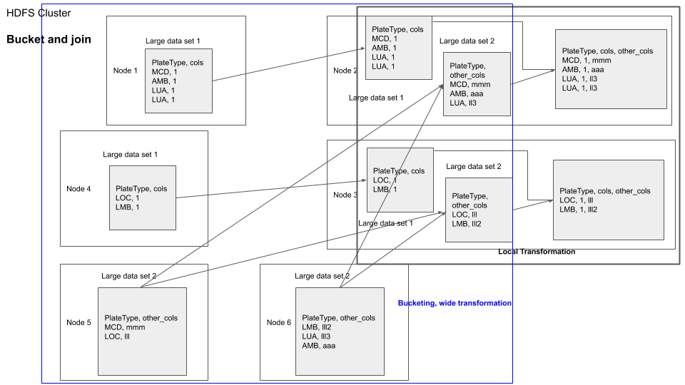
Another approach would be to apply bucketed joins. Bucketing is a technique which you can use to repartition a dataframe based on a field. If you bucket both the dataframe based on the filed that they are supposed to be joined on, it will outcome in both the dataframes having their data chunks to be made bachelor in the same nodes for joins, considering the location of nodes are chosen using the hash of the sectionalisation field.

You can visualize bucketed join every bit shown below

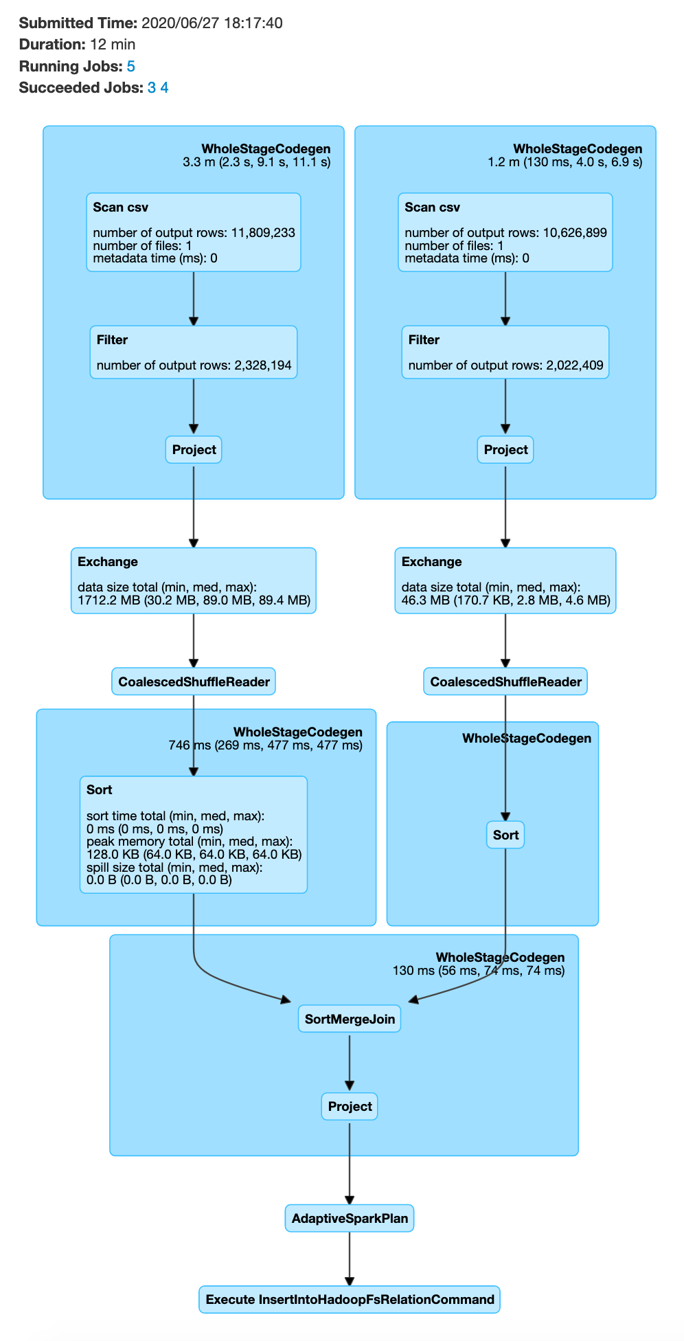
            hdfs dfs -rm -r /output              # free upward some space in HDFS              pyspark --num-executors=              2              --executor-memory=8g              # offset pyspark beat out                      

            parkViolations_2015              =              spark.read.pick("header", True).csv("/input/2015.csv") parkViolations_2016              =              spark.read.selection("header", Truthful).csv("/input/2016.csv")  new_column_name_list=              list(map(lambda              10: x.replace(" ",              "_"), parkViolations_2015.columns))  parkViolations_2015              =              parkViolations_2015.toDF(*new_column_name_list) parkViolations_2015              =              parkViolations_2015.filter(parkViolations_2015.Plate_Type              ==              "COM").filter(parkViolations_2015.Vehicle_Year              ==              "2001") parkViolations_2016              =              parkViolations_2016.toDF(*new_column_name_list) parkViolations_2016              =              parkViolations_2016.filter(parkViolations_2016.Plate_Type              ==              "COM").filter(parkViolations_2016.Vehicle_Year              ==              "2001")              # we filter for COM and 2001 to limit fourth dimension taken for the join              spark.conf.fix("spark.sql.autoBroadcastJoinThreshold",              -              one)              # we practise this then that Spark does not car optimize for circulate bring together, setting to -one ways disable              parkViolations_2015.write.way("overwrite").bucketBy(400,              "Vehicle_Year",              "plate_type").saveAsTable("parkViolations_bkt_2015") parkViolations_2016.write.mode("overwrite").bucketBy(400,              "Vehicle_Year",              "plate_type").saveAsTable("parkViolations_bkt_2016")  parkViolations_2015_tbl              =              spark.read.table("parkViolations_bkt_2015") parkViolations_2016_tbl              =              spark.read.table("parkViolations_bkt_2016")  joinDF              =              parkViolations_2015_tbl.join(parkViolations_2016_tbl, (parkViolations_2015_tbl.Plate_Type              ==              parkViolations_2016_tbl.Plate_Type)              &              (parkViolations_2015_tbl.Vehicle_Year              ==              parkViolations_2016_tbl.Vehicle_Year) ,              "inner").select(parkViolations_2015_tbl["Summons_Number"], parkViolations_2016_tbl["Issue_Date"])  joinDF.explain()              # you lot volition meet SortMergeJoin, but no exchange, which means no information shuffle              # The below join will take a while, approx 30min              joinDF.write.format("com.databricks.spark.csv").choice("header", True).mode("overwrite").save("/output/bkt_joined_df.csv") leave()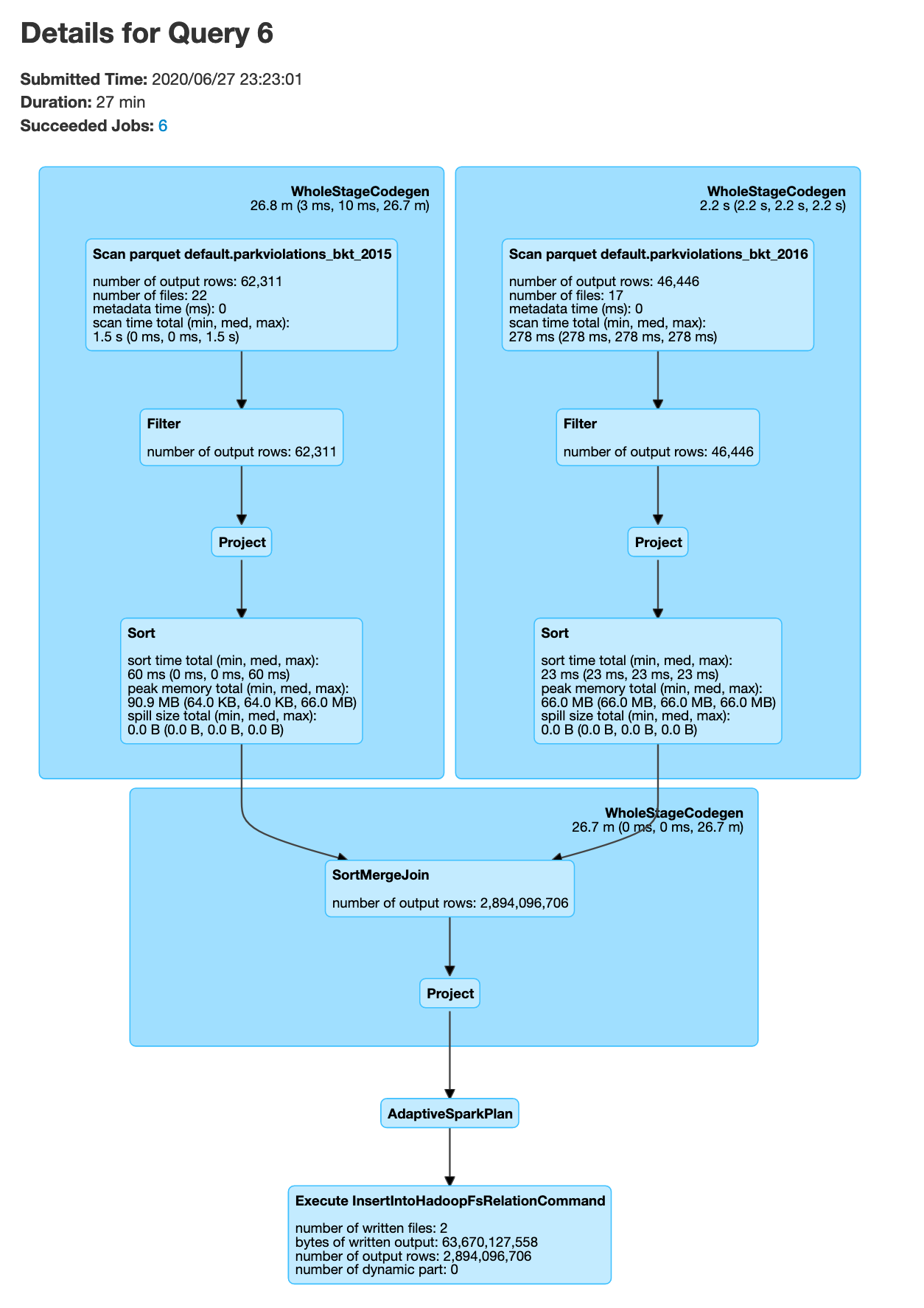                      

Note that in the above lawmaking snippet we kickoff pyspark with --executor-memory=8g this option is to ensure that the memory size for each node is 8GB due to the fact that this is a big join. The number of buckets 400 was chosen to exist an arbritray big number.

The write.bucketBy writes to our HDFS at /user/spark/warehouse/. You can check this using

            hdfs dfs -ls /user/spark/warehouse/                      

user exercise

Effort bucketed join only with different bucket sizes > 400 and < 400. How does information technology touch performance? Why? Tin yous use repartition to achieve same or similar result? If you execute the write in the bucketed tables instance you will notice there will b e one executor at the end that takes upward most of the time, why is this? how can information technology be prevented?

Key points

1. If ane of your table is much smaller compared to the other, consider using broadcast bring together
2. If you want to avoid data shuffle during the join query time, only are ok with pre shuffling the information, consider using the bucketed bring together technique.
3. Bucketing increases performance with discrete columns(ie columns with limited number of unique values, in our instance the plate type cavalcade has 87 distinct values), if the values are continuous(or have loftier number of unique values) the performance boost may non be worth it.

TL; DR

1. Reduce data shuffle, employ repartition to organize dataframes to forestall multiple data shuffles.
2. Use caching, when necessary to continue information in memory to save on disk read costs.
3. Optimize joins to prevent data shuffles, using circulate technique or bucket join techniques.
4. There is no one size fits all solution for optimizing Spark, utilise the above techniques to choose the optimal strategy for your use case.

Conclusion

These are some techniques that help you resolve nearly(usually fourscore%) of your Apache Spark performance issues. Knowing when to use them and when not to use them is crucial, eg. you might not want to utilise caching if that data frame is used for only one transformation. There are more techniques like central salting for dealing with information skew, etc. Simply the key concept is to brand a tradeoff betwixt preprocessing the information to prevent data shuffles so performing transformations equally necessary depending on your use case.

Promise this postal service provides you some means to think almost optimizing your spark lawmaking. Please let me know if yous have whatever questions or comments in the comment section below.

Reference:

1. Spark Docs
2. Bucketing
3. Data

How To Process Over Size Data In Spark,

Source: https://www.startdataengineering.com/post/how-to-optimize-your-spark-jobs/

Posted by: guanplakend.blogspot.com

Share this post